Deep learning has been touted for its potential to enhance the diagnosis of diseases, and now a team of researchers at Stanford has developed a deep-learning algorithm that may make this vision a reality for skin cancer.*
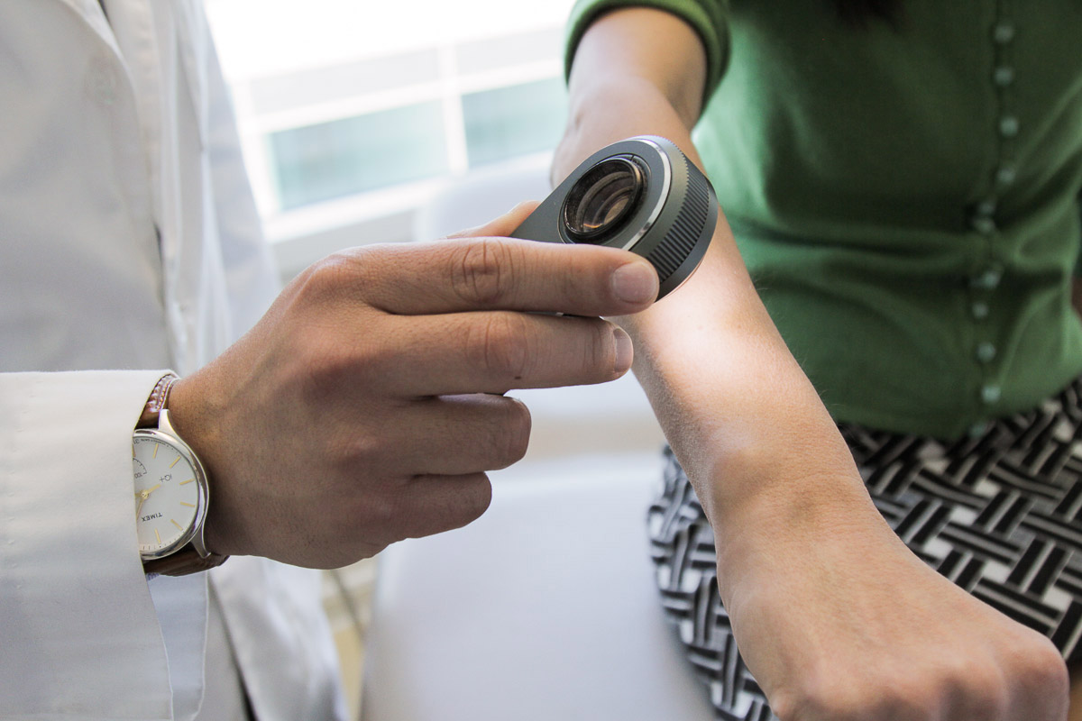
A dermatologist uses a dermatoscope, a type of handheld microscope, to look at skin. Stanford AI scientists have created a deep convolutional neural network algorithm for skin cancer that matched the performance of board-certified dermatologists. (credit: Matt Young)
The researchers, led by Dr. Sebastian Thrun, an adjunct professor at the Stanford Artificial Intelligence Laboratory, reported in the January 25 issue of Nature that their deep convolutional neural network (CNN) algorithm performed as well or better than 21 board-certified dermatologists at diagnosing skin cancer. (See “Skin cancer classification performance of the CNN (blue) and dermatologists (red)” figure below.)
Diagnosing skin cancer begins with a visual examination. A dermatologist usually looks at the suspicious lesion with the naked eye and with the aid of a dermatoscope, which is a handheld microscope that provides low-level magnification of the skin. If these methods are inconclusive or lead the dermatologist to believe the lesion is cancerous, a biopsy is the next step. This deep learning algorithm may help dermatologists decide which skin lesions to biopsy.
“My main eureka moment was when I realized just how ubiquitous smartphones will be,” said Stanford Department of Electrical Engineering’s Andre Esteva, co-lead author of the study. “Everyone will have a supercomputer in their pockets with a number of sensors in it, including a camera. What if we could use it to visually screen for skin cancer? Or other ailments?”
It is projected that there will be 6.3 billion smartphone subscriptionst by the year 2021, according to Ericsson Mobility Report (2016), which could potentially provide low-cost universal access to vital diagnostic care.
Creating the deep convolutional neural network (CNN) algorithm

Deep CNN classification technique. Data flow is from left to right: an image of a skin lesion (for example, melanoma) is sequentially warped into a probability distribution over clinical classes of skin disease using Google Inception v3 CNN architecture pretrained on the ImageNet dataset (1.28 million images over 1,000 generic object classes) and fine-tuned on the team’s own dataset of 129,450 skin lesions comprising 2,032 different diseases. (credit: Andre Esteva et al./Nature)
Rather than building an algorithm from scratch, the researchers began with an algorithm developed by Google that was already trained to identify 1.28 million images from 1,000 object categories. It was designed primarily to be able to differentiate cats from dogs, but the researchers needed it to differentiate benign and malignant lesions. So they collaborated with dermatologists at Stanford Medicine, as well as Helen M. Blau, professor of microbiology and immunology at Stanford and co-author of the paper.
The algorithm was trained with nearly 130,000 images representing more than 2,000 different diseases with an associated disease label, allowing the system to overcome variations in angle, lighting, and zoom. The algorithm was then tested against 1,942 images of skin that were digitally annotated with biopsy-proven diagnoses of skin cancer. Overall, the algorithm identified the vast majority of cancer cases with accuracy rates that were similar to expert clinical dermatologists.
However, during testing, the researchers used only high-quality, biopsy-confirmed images provided by the University of Edinburgh and the International Skin Imaging Collaboration Project that represented the most common and deadliest skin cancers — malignant carcinomas and malignant melanomas.
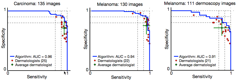
Skin cancer classification performance of the CNN (blue) and dermatologists (red).** (credit: Andre Esteva et al./Nature)
The 21 dermatologists were asked whether, based on each image, they would proceed with biopsy or treatment, or reassure the patient. The researchers evaluated success by how well the dermatologists were able to correctly diagnose both cancerous and non-cancerous lesions in more than 370 images.***
However, Susan Swetter, professor of dermatology and director of the Pigmented Lesion and Melanoma Program at the Stanford Cancer Institute and co-author of the paper, notes that “rigorous prospective validation of the algorithm is necessary before it can be implemented in clinical practice, by practitioners and patients alike.”
* Every year there are about 5.4 million new cases of skin cancer in the United States, and while the five-year survival rate for melanoma detected in its earliest states is around 97 percent, that drops to approximately 14 percent if it’s detected in its latest stages.
*** The algorithm’s performance was measured through the creation of a sensitivity-specificity curve, where sensitivity represented its ability to correctly identify malignant lesions and specificity represented its ability to correctly identify benign lesions. It was assessed through three key diagnostic tasks: keratinocyte carcinoma classification, melanoma classification, and melanoma classification when viewed using dermoscopy. In all three tasks, the algorithm matched the performance of the dermatologists with the area under the sensitivity-specificity curve amounting to at least 91 percent of the total area of the graph. An added advantage of the algorithm is that, unlike a person, the algorithm can be made more or less sensitive, allowing the researchers to tune its response depending on what they want it to assess. This ability to alter the sensitivity hints at the depth and complexity of this algorithm. The underlying architecture of seemingly irrelevant photos — including cats and dogs — helps it better evaluate the skin lesion images.
Abstract of Dermatologist-level classification of skin cancer with deep neural networks
Skin cancer, the most common human malignancy, is primarily diagnosed visually, beginning with an initial clinical screening and followed potentially by dermoscopic analysis, a biopsy and histopathological examination. Automated classification of skin lesions using images is a challenging task owing to the fine-grained variability in the appearance of skin lesions. Deep convolutional neural networks (CNNs) show potential for general and highly variable tasks across many fine-grained object categories. Here we demonstrate classification of skin lesions using a single CNN, trained end-to-end from images directly, using only pixels and disease labels as inputs. We train a CNN using a dataset of 129,450 clinical images—two orders of magnitude larger than previous datasets—consisting of 2,032 different diseases. We test its performance against 21 board-certified dermatologists on biopsy-proven clinical images with two critical binary classification use cases: keratinocyte carcinomas versus benign seborrheic keratoses; and malignant melanomas versus benign nevi. The first case represents the identification of the most common cancers, the second represents the identification of the deadliest skin cancer. The CNN achieves performance on par with all tested experts across both tasks, demonstrating an artificial intelligence capable of classifying skin cancer with a level of competence comparable to dermatologists. Outfitted with deep neural networks, mobile devices can potentially extend the reach of dermatologists outside of the clinic. It is projected that 6.3 billion smartphone subscriptions will exist by the year 2021 and can therefore potentially provide low-cost universal access to vital diagnostic care.
references:
- http://www.nature.com/nature/journal/vaop/ncurrent/full/nature21056.html
